Looking into BrainXcan database
1 About
In this post, we will look into the BrainXcan database and learn about how to load the following data into R:
- Prediction models
- Genotype covariance
- IDP GWASs
These data loading rely on python packages pandas and scipy.sparse which has been installed as part of brainxcan conda environment. To use them in R, we can use reticulate.
The naming convention of IDP is IDP-[UKB_Field_ID] and we call it IDP ID. The information of the IDPs can be found at here.
# load reticulate since we want to use python package
library(reticulate)
## Warning: package 'reticulate' was built under R version 3.6.2# use brainxcan conda env
use_condaenv('brainxcan')
# load python packages
pd = import('pandas')
sp = import('scipy.sparse')2 Prediction models
We share prediction models of original IDPs and residual IDPs trained from ridge and elastic net. The residual IDPs are obtained by regressing out the first principal component of IDP matrix (by subtype) from the original IDP.
For each set of models, strutural IDPs and diffusion IDPs are saved separately and there are two types of files:
*.parquet*.perf.tsv.gz
The parquet file contains the prediction model weights where SNPs are in rows and IDPs are in columns The prediction performance (obtained from training pipeline) of the models is in the tsv.gz file. If setting the number of rows in tsv.gz file as n, then the number of columns in the parquet is n + 4 with the four additional columns indicating: rsID (snpid), non effect allele (a0), effect allele (a1), and chromosome (chr).
The naming rule is:
path-to-brainxcan_data/idp_weights/[model_type]/[idp_type].[modality].*model_type:ridgeorelastic_netidp_type:residualororiginalmodality:dmriort1
Let’s take a look at them.
# set up the file path
model_type = 'ridge'
idp_type = 'residual'
modality = 'dmri'
parquet_file = paste0('idp_weights/', model_type, '/', idp_type, '.', modality, '.parquet')
perf_file = paste0('idp_weights/', model_type, '/', idp_type, '.', modality, '.perf.tsv.gz')
model_type = ridge
idp_type = residual
modality = dmri
Reading parquet file: path-to-brainxcan_data/idp_weights/ridge/residual.dmri.parquet
Reading performance file: path-to-brainxcan_data/idp_weights/ridge/residual.dmri.perf.tsv.gz
# load the parquet file
df_weights = pd$read_parquet(paste0(datadir, '/', parquet_file))
# load the performance file
df_perf = read.table(paste0(datadir, '/', perf_file), stringsAsFactors = F, header = T)

# look at the first 6 columns and rows
head(df_weights[, 1: 6]) %>% pander| snpid | a0 | a1 | chr | IDP-25650 | IDP-25651 |
|---|---|---|---|---|---|
| rs3131972 | A | G | 1 | -3.915e-05 | 6.14e-05 |
| rs3131969 | A | G | 1 | -7.533e-05 | 4.303e-05 |
| rs3131967 | T | C | 1 | -7.558e-05 | 4.256e-05 |
| rs1048488 | C | T | 1 | -3.991e-05 | 5.655e-05 |
| rs12562034 | A | G | 1 | -7.253e-07 | -7.05e-05 |
| rs12124819 | G | A | 1 | -3.426e-06 | 1.991e-05 |
head(df_perf) %>% pander| R2 | Pearson | Spearman | phenotype |
|---|---|---|---|
| 0.01224 | 0.1107 | 0.1094 | IDP-25650 |
| 0.01266 | 0.1125 | 0.1102 | IDP-25651 |
| 0.02177 | 0.1476 | 0.1409 | IDP-25652 |
| 0.01806 | 0.1346 | 0.1313 | IDP-25653 |
| 0.01723 | 0.1325 | 0.1285 | IDP-25654 |
| 0.02 | 0.143 | 0.1363 | IDP-25655 |
Number of rows in weights table = 1071343
Number of columns in weights table = 312
Number of rows in performance table = 308
The parquet file support reading by column. So, if we only want to load the weights of a specific IDP, we can do the following:
idp_id = 'IDP-25652'
df_weights_sub = pd$read_parquet(
  paste0(datadir, '/', parquet_file),
  columns = c('snpid', 'a0', 'a1', 'chr', idp_id)
)
df_weights_sub %>% head %>% pander| snpid | a0 | a1 | chr | IDP-25652 |
|---|---|---|---|---|
| rs3131972 | A | G | 1 | 2.21e-06 |
| rs3131969 | A | G | 1 | 1.576e-05 |
| rs3131967 | T | C | 1 | 1.627e-05 |
| rs1048488 | C | T | 1 | 4.518e-06 |
| rs12562034 | A | G | 1 | -0.0001214 |
| rs12124819 | G | A | 1 | -4.941e-05 |
3 Genotype covariance
Genotype covariance was computed using the UKB IDP cohort (the same as prediction model training). The genotype covariance is saved by chromosome. It is a banded matrix with the band width = 200 and only the upper triangular values are saved since it is symmetric. These genotype covariance files are at brainxcan_data/geno_covar/ and for each chromosome, there are two files:
chr*.banded.npz: The banded genotype covariance in scipy sparse matrix format.chr*.banded.snp_meta.parquet: The meta data annotating the rows/columns of the genotype covariance file in parquet format. The number of rows of the meta data matches the genotype covariance file and the SNPs are in the same order.
# load banded genotype covariance
mat = sp$load_npz(paste0(datadir, '/geno_covar/chr22.banded.npz'))

# take the first 500 SNPs and visualize
mat_sub = as.matrix(mat[ 1 : 500, 1 : 500])
var_sub = diag(mat_sub)
cor_sub = sweep(mat_sub, 1, FUN = '/', sqrt(var_sub))
cor_sub = sweep(cor_sub, 2, FUN = '/', sqrt(var_sub))
par(mfrow = c(1, 2))
image(mat_sub, main = 'Covariance between SNPs')
image(cor_sub, main = 'Correlation between SNPs')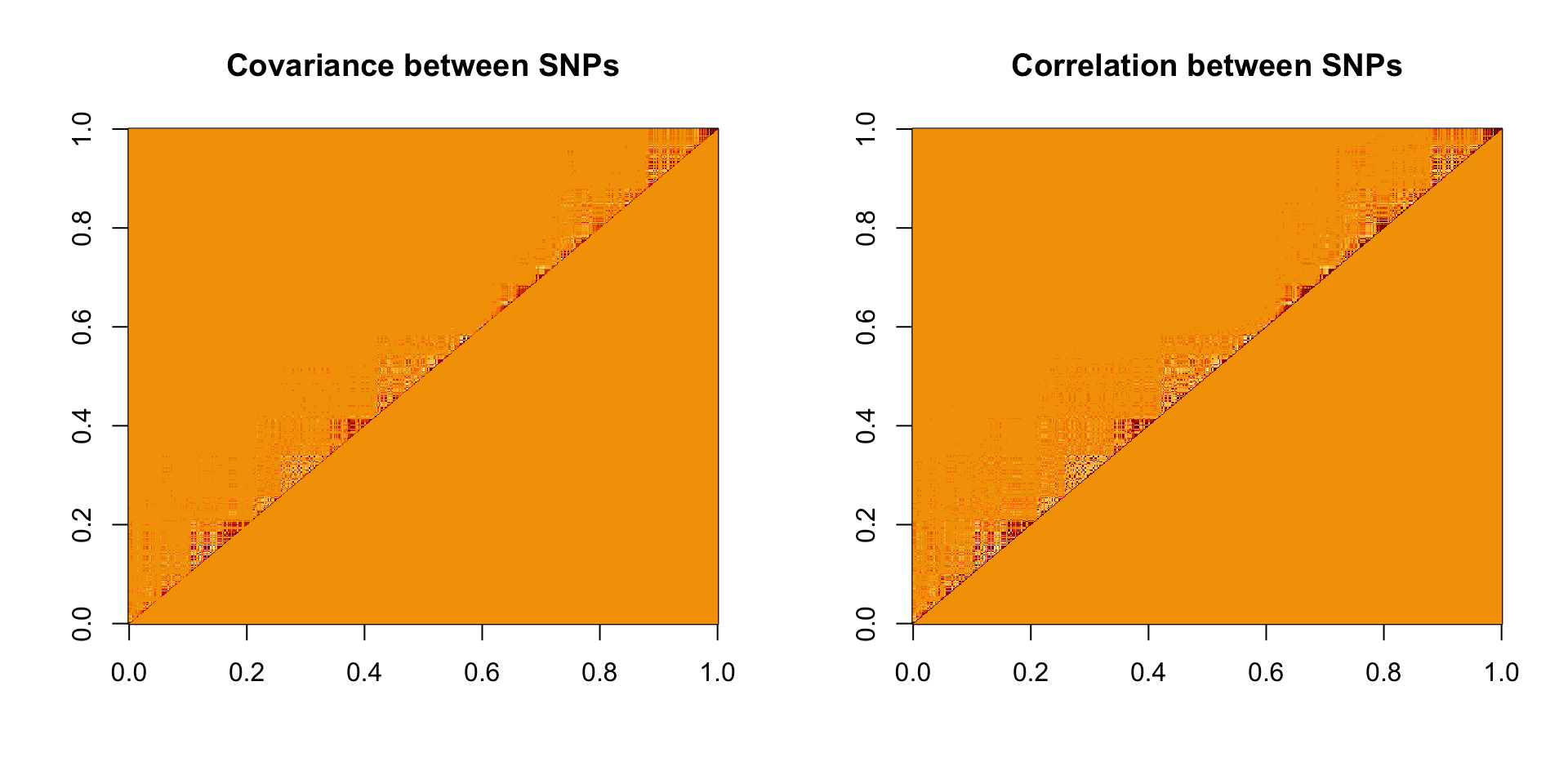
class(mat) = dgTMatrix
To annotate the genotype covariance with the actual SNP information, we should load the meta data.
df_snp = pd$read_parquet(paste0(datadir, '/geno_covar/chr22.banded.snp_meta.parquet'))
df_snp %>% head %>% pander| snpid | effect_allele | non_effect_allele | chr |
|---|---|---|---|
| rs7287144 | G | A | 22 |
| rs5748662 | A | G | 22 |
| rs5747620 | C | T | 22 |
| rs9605903 | C | T | 22 |
| rs5746647 | G | T | 22 |
| rs16980739 | T | C | 22 |
Number of rows in meta data = 15747
Number of rows/columns in genotype covariance = 15747, 15747
4 IDP GWAS
We share the IDP GWAS results for all the IDPs being analyzed and the study cohort is the same as IDP model training (n = 24,490).
The GWAS results are by chromosome and by IDP and the naming rule is as follow:
path-to-brainxcan_data/idp_gwas/[idp_type].[modality].chr[chr_num]/[idp_id]].parquetidp_type:residualororiginalmodality:dmriort1chr_num: 1 to 22idp_id: IDP ID
The SNPs are in rows and columns are:
variant_id: rsID of the SNPphenotype_id: IDP IDpval: P-value of the associationbandb_se: Estimated effect size and standard errormaf: Minor allele frequency of the SNP in the GWAS cohort
Further annotation of the SNPs can be found at path-to-brainxcan_data/idp_gwas/snp_bim/chr[chr_num].bim. This is essentially PLINK BIM file and the columns are: 1. Chromosome, 2. rsID, 3. placeholder, 4. Genomic position, 5. Effect allele, 6. Non-effect allele. The GWAS direction is the same as the one in BIM file.
For instance, let’s load one GWAS file.
# set up the file path
idp_type = 'residual'
modality = 't1'
chr_num = 22
idp_id = 'IDP-25002'
gwas_file = paste0('idp_gwas/', idp_type, '.', modality, '.chr', chr_num, '/', idp_id, '.parquet')
bim_file = paste0('idp_gwas/', 'snp_bim/', 'chr', chr_num, '.bim')
idp_type = residual
modality = t1
chr_num = 22
idp_id = IDP-25002
Reading parquet file: path-to-brainxcan_data/idp_gwas/residual.t1.chr22/IDP-25002.parquet
Reading BIM file: path-to-brainxcan_data/idp_gwas/snp_bim/chr22.bim
df_gwas = pd$read_parquet(paste0(datadir, '/', gwas_file))
df_bim = read.table(
  paste0(datadir, '/', bim_file),
  col.names = c('chromosome', 'variant_id', 'ph', 'position', 'effect_allele', 'non_effect_allele'),
  stringsAsFactors = F
) %>% select(-ph)  # remove placeholder column

# annotate GWAS results with additional SNP information
df_gwas = right_join(df_bim, df_gwas, by = 'variant_id')

df_gwas %>% mutate(position = as.character(position)) %>% head %>% pander| chromosome | variant_id | position | effect_allele | non_effect_allele | phenotype_id | pval | b | b_se | maf |
|---|---|---|---|---|---|---|---|---|---|
| 22 | rs4911642 | 16504399 | C | T | IDP-25002 | 0.3064 | -0.02878 | 0.02814 | 0.08711 |
| 22 | rs7287144 | 16886873 | G | A | IDP-25002 | 0.7055 | 0.003934 | 0.01041 | 0.2708 |
| 22 | rs5748662 | 16892858 | A | G | IDP-25002 | 0.6634 | 0.00454 | 0.01043 | 0.2699 |
| 22 | rs2027653 | 16918335 | T | C | IDP-25002 | 0.573 | -0.01169 | 0.02074 | 0.425 |
| 22 | rs9680776 | 17000277 | T | C | IDP-25002 | 0.8555 | 0.003334 | 0.0183 | 0.1795 |
| 22 | rs5747620 | 17032698 | C | T | IDP-25002 | 0.2179 | 0.01388 | 0.01127 | 0.4 |