4.1 Load summary files

filenames = 1 : 3
summary_table <- c()
for(i in filenames){
    temp <- read.table(paste('../data/040417_overnight/', paste(i, 'csv', sep = '.'), sep = ''), sep = ',', header = T)
    temp$repeatID <- rep(i, nrow(temp))
    summary_table <- rbind(summary_table, temp)
}

4.2 Loss and validation loss

library(ggplot2)
ggplot() + geom_line(data = summary_table[summary_table$variable == 'loss',], aes(x = epoch, y = value, group = repeatID, color = 'loss')) + geom_line(data = summary_table[summary_table$variable == 'val_loss',], aes(x = epoch, y = value, group = repeatID, color = 'val_loss')) + ggtitle('Loss and validation loss along the optimization')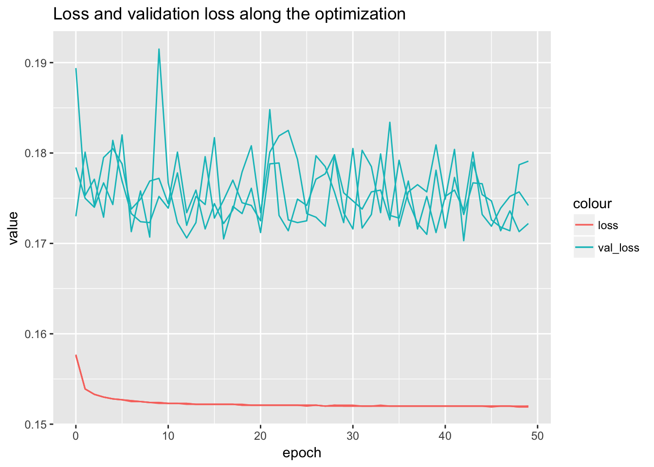

4.3 Precision, recall, and AUCs

temp <- summary_table[!summary_table$variable %in% c('loss', 'val_loss'), ]
temp$type <- factor(temp$variable, levels = c('cross_entropy', 'roc_auc', 'pr_auc', 'accuracy', 'precision_f', 'precision_t', 'recall_f', 'recall_t', 'proportion_f', 'proportion_t'))
ggplot(temp) + geom_boxplot(aes(x = type, y = value, color = data)) + theme(axis.text.x = element_text(angle = 30, hjust = 1)) + ggtitle('Performance overview')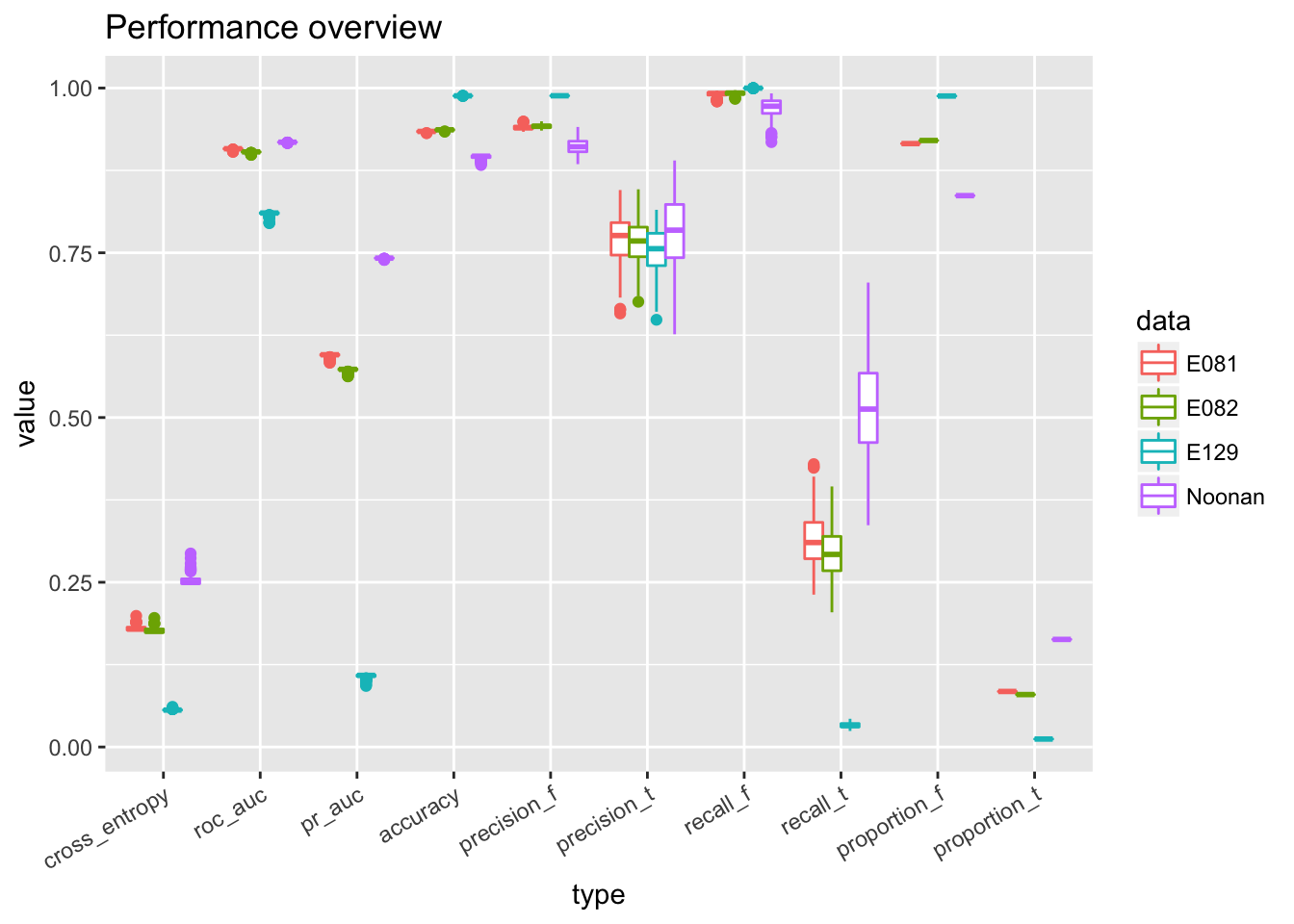

temp.no_proportion <- temp[!grepl('proportion', temp$type), ]
ggplot(temp.no_proportion[temp.no_proportion$data == 'Noonan',]) + geom_line(aes(x = epoch, y = value, group = repeatID)) + facet_grid(type ~ ., scales = 'free_y', ) + ggtitle('Noonan H3K27ac') + theme(strip.text.y = element_text(angle = 0))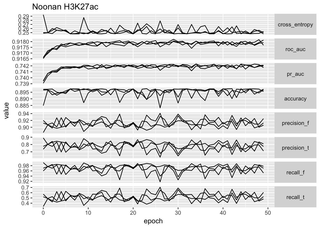

ggplot(temp.no_proportion[temp.no_proportion$data == 'E129',]) + geom_line(aes(x = epoch, y = value, group = repeatID)) + facet_grid(type ~ ., scales = 'free_y', ) + ggtitle('E129 H3K9me3') + theme(strip.text.y = element_text(angle = 0))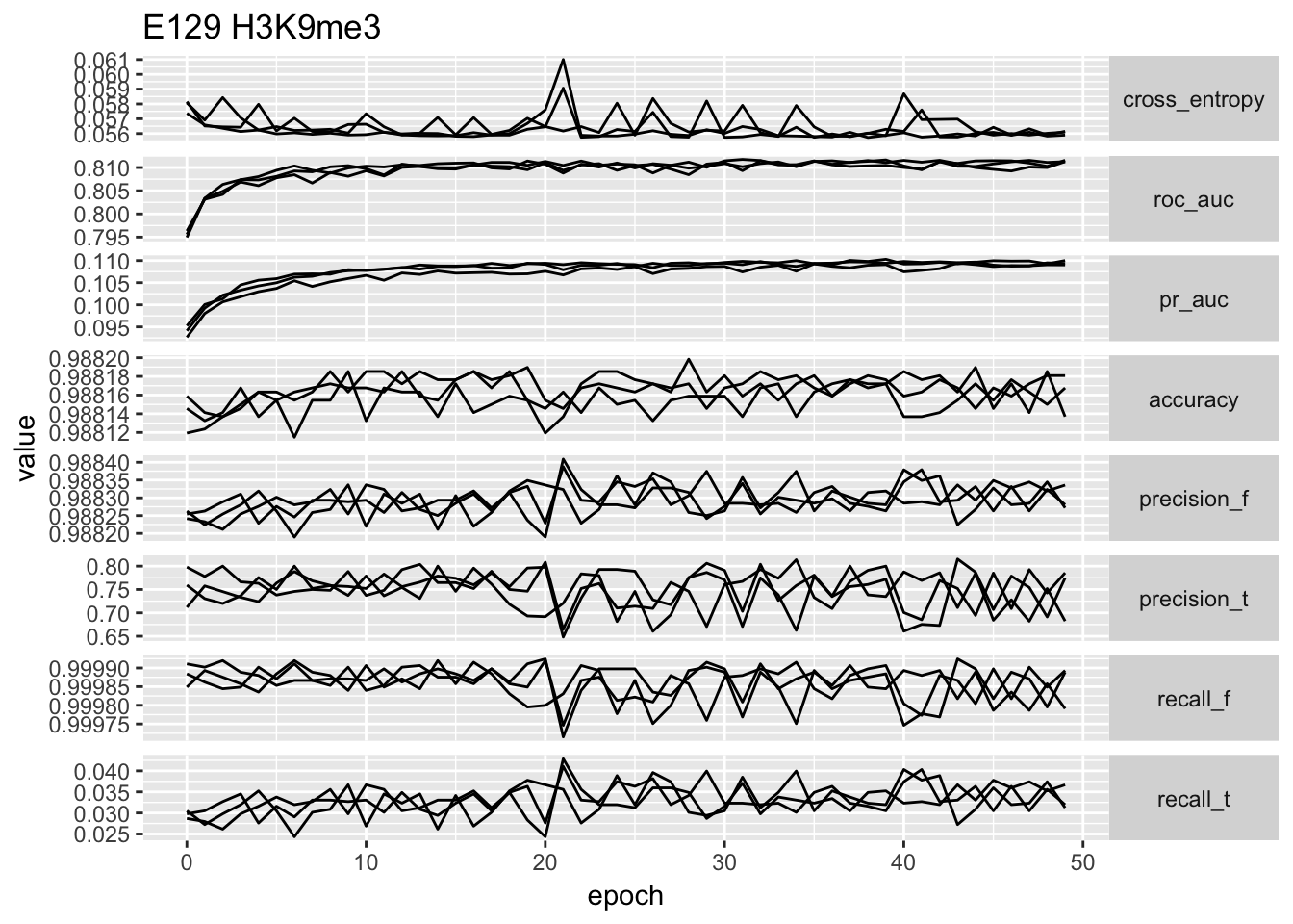

ggplot(temp.no_proportion[temp.no_proportion$data == 'E081',]) + geom_line(aes(x = epoch, y = value, group = repeatID)) + facet_grid(type ~ ., scales = 'free_y', ) + ggtitle('E081 DNase') + theme(strip.text.y = element_text(angle = 0))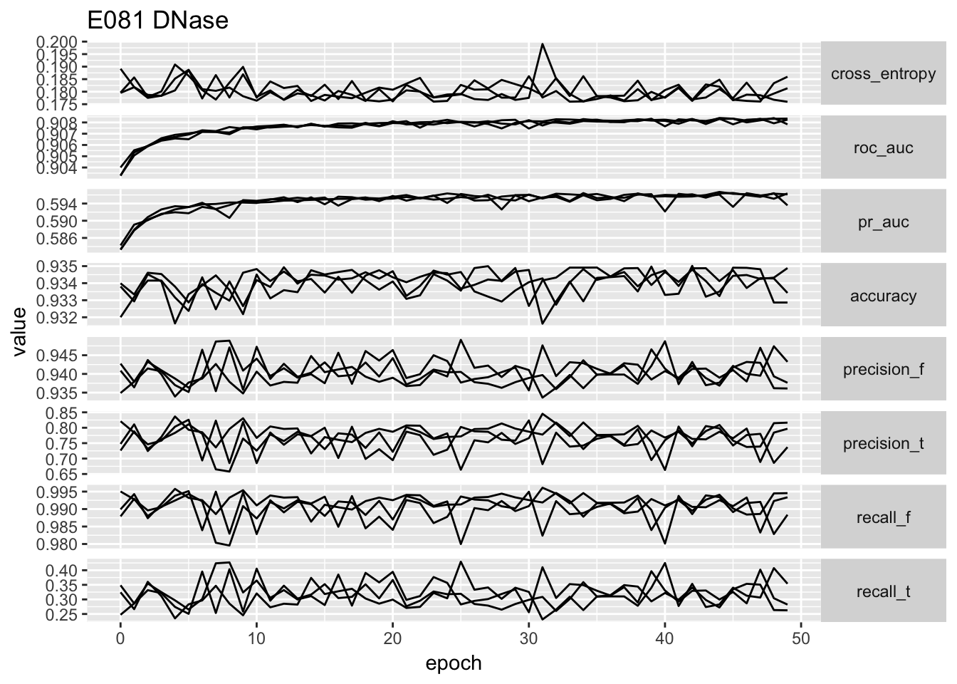

ggplot(temp.no_proportion[temp.no_proportion$data == 'E082',]) + geom_line(aes(x = epoch, y = value, group = repeatID)) + facet_grid(type ~ ., scales = 'free_y', ) + ggtitle('E082 DNase') + theme(strip.text.y = element_text(angle = 0))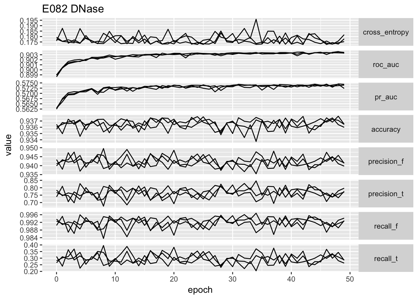

# ggplot(temp) + geom_point(aes(x = cross_entropy, y = roc_auc)) + facet_wrap(~data, scales = 'free')

From the performance curves we can see that the present feature representation works well on E081, E082 DNase data but it works really poorly on Noonan’s H3K27ac data. First of all, the bad performance is hardly due to optimization issue, because we have run 50 epochs and other data sets have reached a reasonable performance. We select the one with lowest validation loss as the best model for down stream analysis.

best_model <- summary_table[summary_table$variable == 'val_loss', ][order(summary_table[summary_table$variable == 'val_loss', ]$value, decreasing = F)[1],]
print(best_model)

##      X data epoch  value variable repeatID
## 4075 0  all    42 0.1703 val_loss        2

temp_dcast <- dcast(temp, epoch + repeatID + data ~ type)
best_model_melted <- temp_dcast[temp_dcast$epoch == best_model$epoch & temp_dcast$repeatID == best_model$repeatID,]
write.table(best_model_melted, file='../data/best_model_type1_scores.txt', sep = '\t', row.names = F, quote = F)

4.4 Compare performance of best model with DeepSEA result

source('~/Box Sync/2017_spring/tasks/deep_variant/DeepSEA/doc/cell_type/yanyu_lib.R')
library(stringr)
aucs_danq <- read.table('../../DeepVariantAnnotation/data/aucs.txt', sep = '\t', header = T)
aucs_danq <- as_num(aucs_danq)

## Warning in as_num(aucs_danq): NAs introduced by coercion

## Warning in as_num(aucs_danq): NAs introduced by coercion

aucs_danq <- aucs_danq[!is.na(aucs_danq$DeepSEA.ROC.AUC),]
aucs_danq$AnnotationType <- to_annotation_type(aucs_danq$TF.DNase.HistoneMark)
temp_data <- aucs_danq[aucs_danq$AnnotationType == 'DNase',]
p1<-ggplot(aucs_danq) + geom_histogram(aes(x = DeepSEA.ROC.AUC, fill = AnnotationType), bins=50) + facet_grid(AnnotationType~., scales = 'free_y') + theme(strip.background = element_blank(), strip.text.y = element_blank(),legend.position="none") + scale_x_continuous(limits=c(0.25, 1))
p2<-ggplot(aucs_danq) + geom_histogram(aes(x = DeepSEA.PR.AUC, fill = AnnotationType), bins=30) + facet_grid(.~AnnotationType, scales = 'free_y') + coord_flip() + theme(strip.background = element_blank(), strip.text.x = element_blank(), legend.position="none")
p3<-ggplot() + geom_point(data = aucs_danq, aes(x = DeepSEA.ROC.AUC, y = DeepSEA.PR.AUC, color = AnnotationType)) + theme( legend.box = "horizontal", legend.justification=c(0,1), legend.position=c(0,1), legend.text=element_text(size=5), legend.title=element_text(size=5)) + geom_point(data = best_model_melted, aes(x = roc_auc, y = pr_auc, shape = data)) + scale_x_continuous(limits=c(0.25, 1))
multiplot(p3, p1, p2, cols=2)

## Warning: Removed 3 rows containing missing values (geom_bar).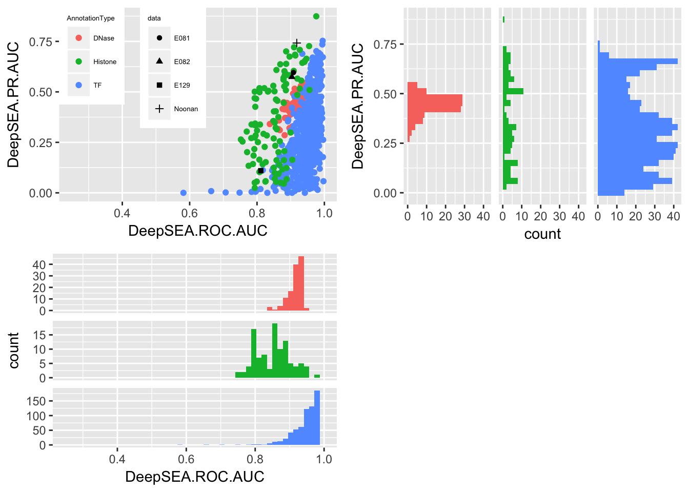

It shows that the result of E081, E082 are compatible to the DNase result in DeepSEA. E129 which is one of the data set in DeepSEA, it achieves similar result as DeepSEA one. But the H3K27ac data behaves poorly, which indicates that the feature representation is not suitable for this data. Another issue is that it is possible that the poor performance data sets have a more unbalanced label set. TODO show that!