rm(list = ls())
library(ggplot2)
theme_set(theme_bw(base_size = 12))
library(dplyr)
library(reshape2)
options(stringsAsFactors = FALSE)
source('../code/rlib_analysis.R')
datadir = '~/Desktop/mixqtl-pipeline-results/simulation-mixqtl'
cbPalette2 <- c("ascQTL" = "#999999", "mixQTL" = "#E69F00", "trcQTL" = "#56B4E9", 'WASP2' = "#009E73", 'RASQUAL' = "#F0E442", 'WASP' = "#0072B2", "#D55E00", "#CC79A7")
source('https://gist.githubusercontent.com/liangyy/43912b3ecab5d10c89f9d4b2669871c9/raw/8151c6fe70e3d4ee43d9ce340ecc0eb65172e616/my_ggplot_theme.R')
th$panel.border = element_rect(colour = th$axis.line$colour)

1 Load data

thetas = c('5e-5', '2.5e-5', '1e-5', '5e-6', '2.5e-6', '1e-6')
samplesizes = (1 : 5) * 100
dat_list = list()
for(theta in thetas) {
  for(samplesize in samplesizes) {
    jobname = paste0('samplesize', samplesize, '_x_', 'theta', theta)
    filename = paste0(datadir, '/', 'mixqtl.', jobname, '__from_1_to_200.txt.gz')
    tmp = read.table(filename, header = T)
    dat_list[[length(dat_list) + 1]] = tmp %>% mutate(theta = theta, sample_size = samplesize)
  }
}
dat = do.call(rbind, dat_list)
for(i in c('pval.trc', 'pval.asc', 'pval.meta')) {
  dat[, i] = fill_in_na_pval(dat[, i])
}
dat$theta = factor(dat$theta, levels = thetas)

2 Type I error

Calculate type I error at alpha = 0.05.

dat_null = dat %>% filter(beta == 0) %>% mutate(idx = 1 : nrow(.))
melt_null = dat_null %>% melt(id.vars = c('idx', 'theta', 'sample_size'), measure.vars = c('pval.trc', 'pval.asc', 'pval.meta'))
melt_null = melt_null %>% mutate(is_sig = is_sig(value))
summary_t1e = melt_null %>% group_by(theta, sample_size, variable) %>% summarize(t1e = mean(is_sig), nobs = n()) %>% ungroup() %>% mutate(t1e_se = sqrt(t1e * (1 - t1e) / nobs)) 
summary_t1e = summary_t1e %>% mutate(method = add_new_name_by_map(variable, map = data.frame(
  x = c('pval.trc', 'pval.asc', 'pval.meta'),
  y = c('trcQTL', 'ascQTL', 'mixQTL')
)))

Plot the whole grid (for supplement).

p = summary_t1e %>% ggplot(aes(color = method)) + 
  geom_bar(aes(x = method, y = t1e), stat = 'identity', fill = 'white') + 
  geom_errorbar(aes(x = method, ymin = t1e - t1e_se * 1.96, ymax = t1e + t1e_se * 1.96), width = .2) + 
  geom_hline(yintercept = 0.05, linetype = 2) + 
  scale_color_manual(values=cbPalette2) + 
  ggtitle('Type I error') + 
  facet_grid(sample_size~theta)  # , labeller = label_both
p = p + theme(axis.text.x=element_text(angle = 45, hjust = 1, vjust = 1))
p = p + th
p = p + xlab('Method') + ylab('Type I error')
p = p + theme(legend.position = 'bottom') + theme(aspect.ratio = 1)
p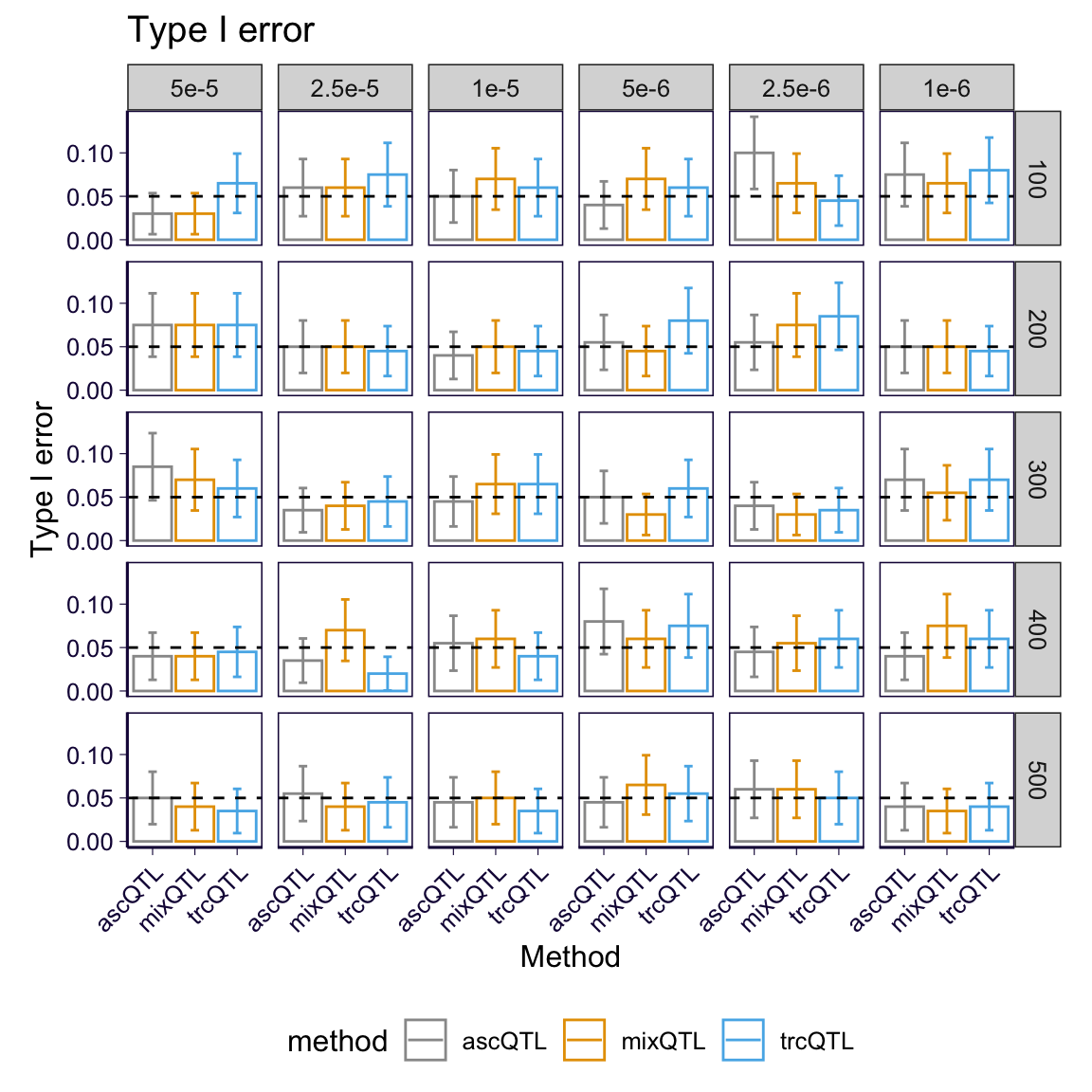

ggsave('../output/grid_sim_0615-matrix_t1e_full.png', p, height = 6, width = 6)

Plot a sub-grid for main text.

sub_thetas = c('1e-5', '2.5e-6')
sub_samplesizes = c(100, 300, 500)
p = summary_t1e %>% filter(theta %in% sub_thetas, sample_size %in% sub_samplesizes) %>% ggplot(aes(color = method)) + 
  geom_bar(aes(x = method, y = t1e), stat = 'identity', fill = 'white') + 
  geom_errorbar(aes(x = method, ymin = t1e - t1e_se * 1.96, ymax = t1e + t1e_se * 1.96), width = .2) + 
  geom_hline(yintercept = 0.05, linetype = 2) + 
  scale_color_manual(values=cbPalette2) + 
  # ggtitle('Type I error') + 
  facet_grid(sample_size~theta, labeller = label_both)
p = p + theme(axis.text.x=element_text(angle = 45, hjust = 1, vjust = 1))
p = p + th
p = p + xlab('Method') + ylab('Type I error')
p = p + theme(legend.position = 'bottom') + theme(aspect.ratio = 1)
p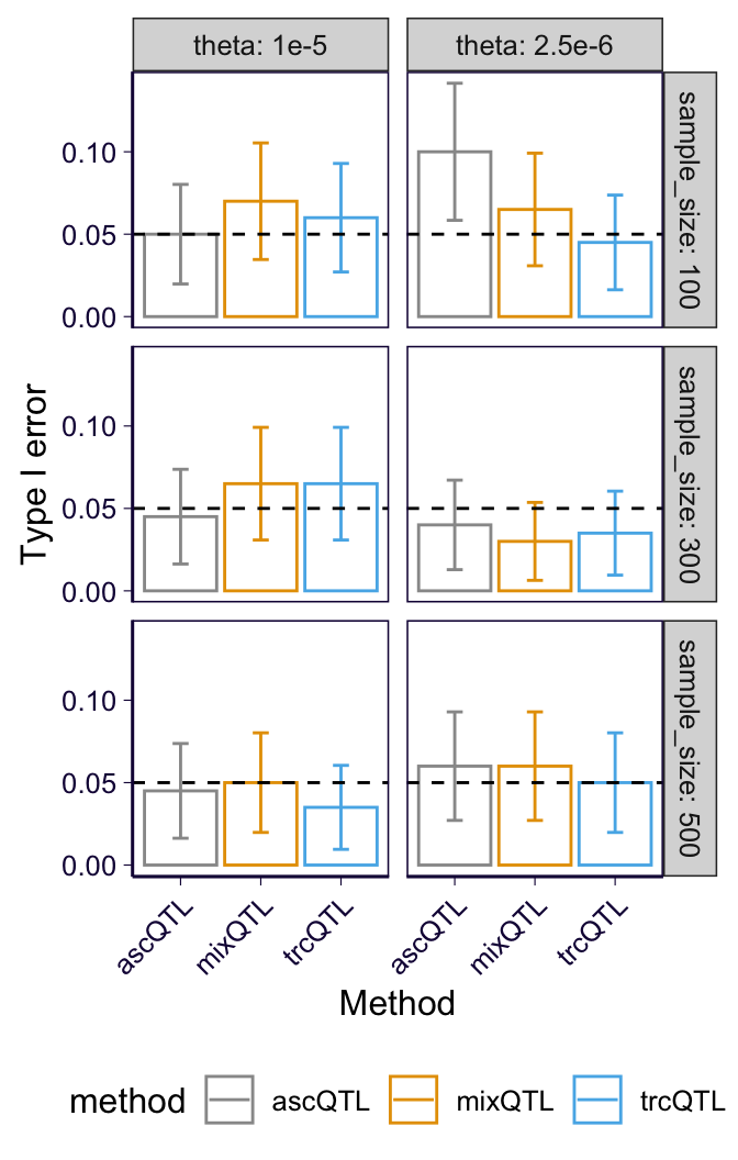

ggsave('../output/grid_sim_0615-matrix_t1e.png', p, height = 5.5, width = 3.5)

3 Power

Calculate power at alpha = 0.05

dat_causal = dat %>% filter(beta != 0) %>% mutate(idx = 1 : nrow(.))
melt_causal = dat_causal %>% melt(id.vars = c('idx', 'theta', 'sample_size', 'beta'), measure.vars = c('pval.trc', 'pval.asc', 'pval.meta'))
melt_causal = melt_causal %>% mutate(is_sig = is_sig(value))
summary_causal = melt_causal %>% group_by(theta, sample_size, variable, beta) %>% summarize(power = mean(is_sig), nobs = n()) %>% ungroup() %>% mutate(power_se = sqrt(power * (1 - power) / nobs)) 
summary_causal = summary_causal %>% mutate(method = add_new_name_by_map(variable, map = data.frame(
  x = c('pval.trc', 'pval.asc', 'pval.meta'),
  y = c('trcQTL', 'ascQTL', 'mixQTL')
)))

Plot the full grid (for supplement)

p = summary_causal %>% mutate(fold_change = exp(beta)) %>% ggplot(aes(color = method)) + 
  geom_point(aes(x = factor(fold_change), y = power), alpha = .5) + 
  geom_line(aes(x = factor(fold_change), y = power, group = method), alpha = .5) + 
  scale_color_manual(values=cbPalette2) + 
  facet_grid(sample_size~theta)
p = p + theme(axis.text.x=element_text(angle = 45, hjust = 1, vjust = 1, size = 8)) # + ggtitle('Power')
p = p + th
p = p + xlab('True aFC') + ylab('Power')
p = p + theme(legend.position = 'bottom') + theme(aspect.ratio = 1)
p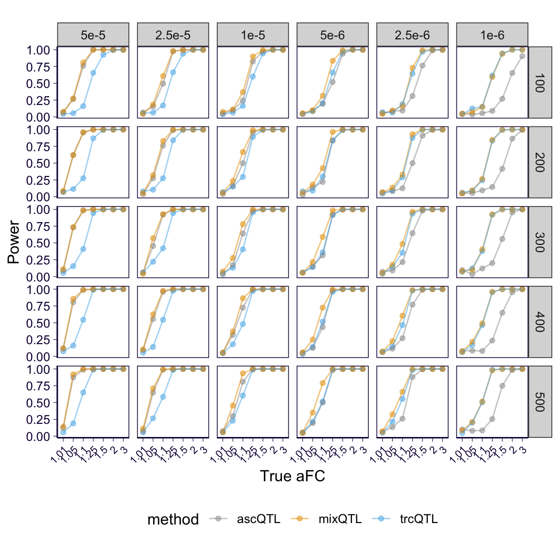

ggsave('../output/grid_sim_0615-matrix_power_full.png', p, height = 6, width = 6)

Plot a sub-grid for main text.

p = summary_causal %>% filter(theta %in% sub_thetas, sample_size %in% sub_samplesizes) %>% mutate(fold_change = exp(beta)) %>% 
  ggplot(aes(color = method)) + 
  geom_point(aes(x = factor(fold_change), y = power), alpha = .5) + 
  geom_line(aes(x = factor(fold_change), y = power, group = method), alpha = .5) +
  scale_color_manual(values=cbPalette2) + 
  facet_grid(sample_size~theta, labeller = label_both)
p = p + theme(axis.text.x=element_text(angle = 45, hjust = 1, vjust = 1)) # + ggtitle('Power')
p = p + th
p = p + xlab('True aFC') + ylab('Power')
p = p + theme(legend.position = 'bottom') + theme(aspect.ratio = 1)
ggsave('../output/grid_sim_0615-matrix_power.png', p, height = 5.5, width = 3.5)

4 Estimates

Organize the data

dat_est = dat %>% mutate(idx = 1 : nrow(.))
melt_est = dat_est %>% melt(id.vars = c('idx', 'theta', 'sample_size', 'beta'), measure.vars = c('bhat.trc', 'bhat.asc', 'bhat.meta'))
melt_est = melt_est %>% mutate(method = add_new_name_by_map(variable, map = data.frame(
  x = c('bhat.trc', 'bhat.asc', 'bhat.meta'),
  y = c('trcQTL', 'ascQTL', 'mixQTL')
)))

Plot the full grid.

p = melt_est %>% filter((round(exp(beta) * 100)) %in% c(100, 110, 200)) %>% mutate(fold_change = exp(beta), fold_change_estimate = exp(value), diff = value - beta) %>% ggplot() + geom_hline(yintercept = 0, color = 'lightgray') + geom_violin(aes(x = factor(fold_change), y = diff, color = method)) + scale_color_manual(values=cbPalette2) + facet_grid(sample_size~theta) # + ggtitle('Estimated effect size')
p = p + theme(axis.text.x=element_text(angle = 45, hjust = .5, vjust = .5))
p = p + th
p = p + theme(legend.position = 'bottom')
p = p + xlab('True aFC') + ylab(expression(hat(beta) - beta[true])) + theme(aspect.ratio = 1) 
p

## Warning: Removed 6 rows containing non-finite values (stat_ydensity).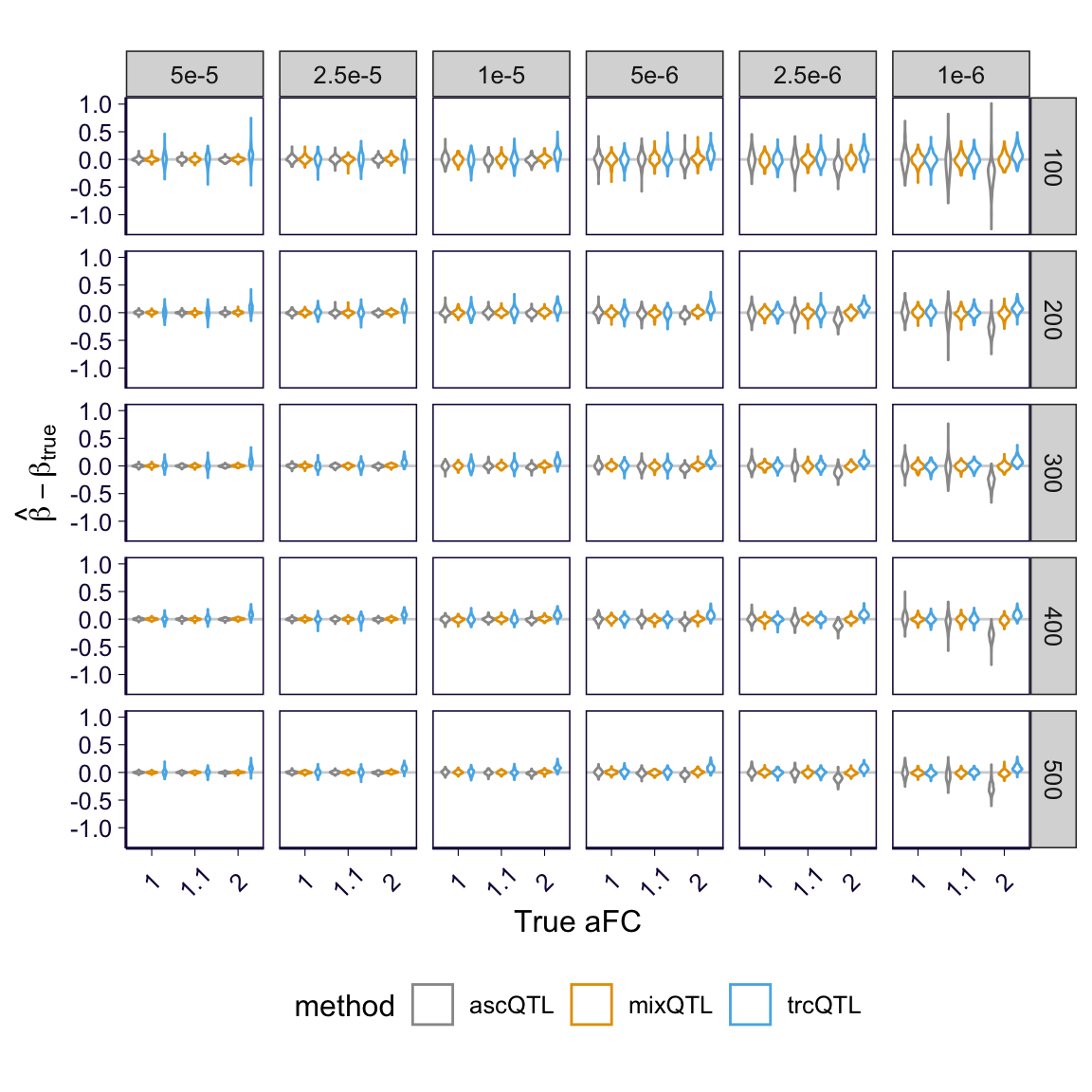

ggsave('../output/grid_sim_0615-matrix_estimate_full.png', p, height = 6, width = 6)

## Warning: Removed 6 rows containing non-finite values (stat_ydensity).

Plot sub-grid for main text.

p = melt_est %>% filter((round(exp(beta) * 100)) %in% c(125, 150, 200, 300)) %>% filter(theta %in% sub_thetas, sample_size %in% sub_samplesizes) %>% mutate(fold_change = exp(beta), fold_change_estimate = exp(value), diff = value - beta) %>% ggplot() + geom_boxplot(aes(x = factor(fold_change), y = fold_change_estimate, color = method)) + scale_color_manual(values=cbPalette2) + geom_point(aes(x = factor(fold_change), fold_change), shape = 3) + facet_grid(sample_size~theta, labeller = label_both) # + ggtitle('Estimated effect size')
p = p + theme(axis.text.x=element_text(angle = 45, hjust = .5, vjust = .5))
p = p + th
p = p + theme(legend.position = 'bottom')
p = p + xlab('True aFC') + ylab('Estimated aFC') + theme(aspect.ratio = 1)
p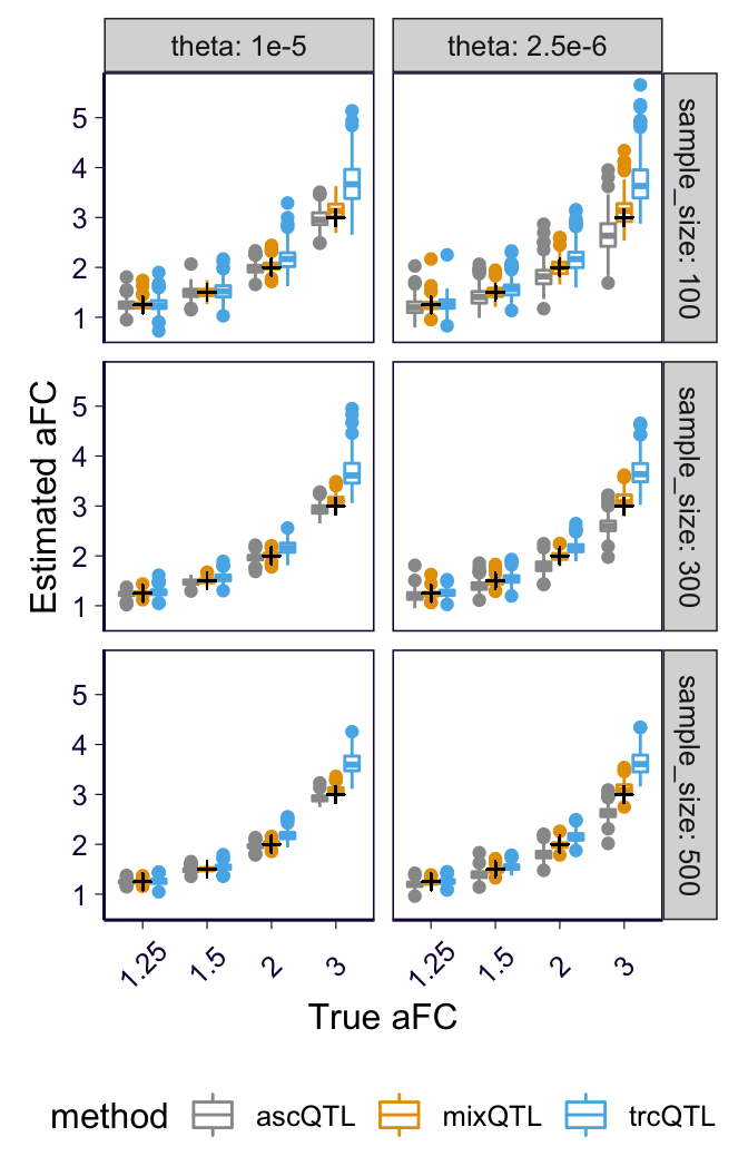

ggsave('../output/grid_sim_0615-matrix_estimate.png', p, height = 5.5, width = 3.5)

Results on mixQTL runs on simulated data

1 Load data

2 Type I error

3 Power

4 Estimates