PennCNV: An integrated hidden Markov model designed for high-resolution copy number variation detection in whole-genome SNP genotyping data
Apr 18, 2018 11:21 · 1787 words · 9 minutes read
\(\newcommand\E{\text{E}}\) \(\newcommand\nocr{\nonumber\\}\)
Meta data of reading
- Journal: Genome research
- Year: 2007
- DOI: 10.1101/gr.6861907
Motivation
This paper calls CNV from genotype microarray data. It is a nice example of how HMM is built up based on how the data is generated (emission) and the underlying process works (transition). For the computation part, since the emission and transition probability is parameterized by some standard distribution and it is different from what is always taught in class (transition matrix and emission matrix), I will briefly discuss the idea behind the Baum-Welch algorithm in this more general set up. Hopefully, this discussion will help to understand B-W algorithm better and from a more general perspective.
Furthermore, this paper also discussed how to incorporate family-based information into the framework. Intuitively, family information constraint the solution probabilistically in the such a way that children CNV event is the result of inheritance and de novo event so that there should be dependency between parent state and child state. So, the Viterbi algorithm needs to be run on sequences in the family jointly.
Observed signal
The genotyping array gives the following signals:
- B allele frequency: This is kind of an extension of genotype. It provides the estimate of the ratio of allele count at the locus
- Log R ratio: This is a measure of the normalized signal intensity
Intuitively, for a normal region with no CNV, BAF is 0, 1/2, 1 and the intensity should be intermediate. For a CNV event (suppose \(k\)), the BAF can take value other than 0, 1/2, 1 and it will be \(i/k\) for \(i = 0, \cdots, k\) instead. Also, the intensity will be different (though it might not follow nice linear relationship). A nice illustration of how BAF and LRR are informative in terms of CNV state is fig 1.
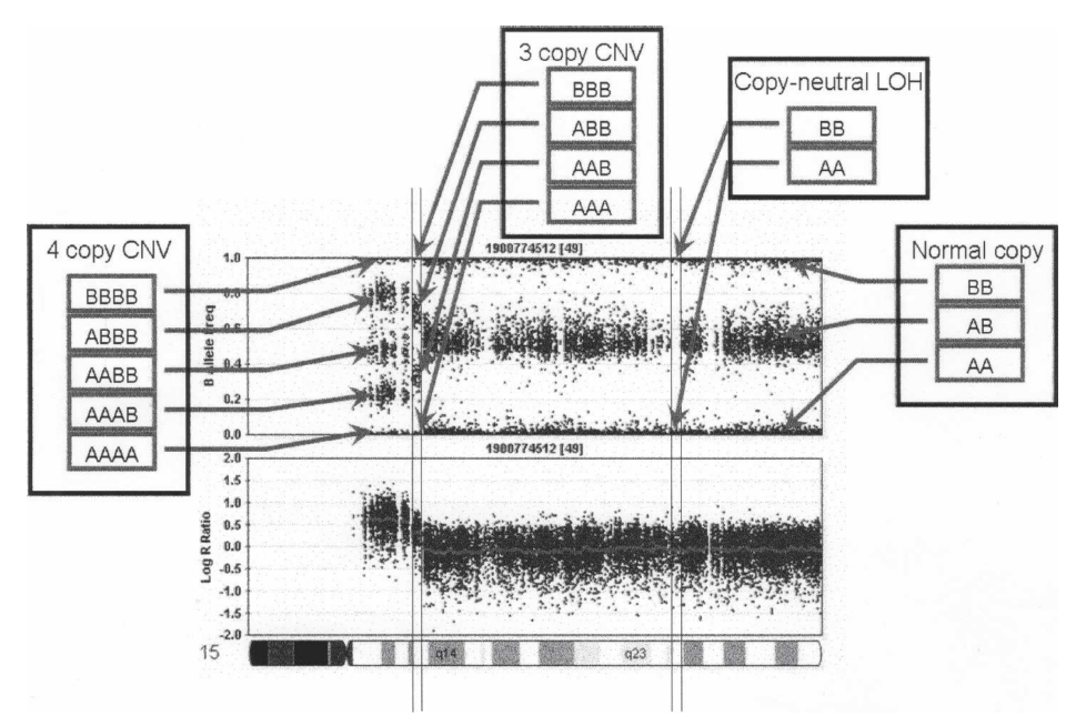
BAF and LRR signals vary among CNV states
Emission probabilities
Following the idea above, it is straight forward to write down the emission probability. Let BAF be \(b\) and LRR be \(r\). \[\begin{align*} \Pr(r | z) &= \pi_r + (1 - \pi_r) N(r; \mu_{r, z}, s_{r, z}) \\ \Pr(b | z) &= \pi_b + (1 - \pi_b) \sum_{g \in G(z)}\Pr(G = g|z)\Pr(b|g) \end{align*}\], where \(G(z)\) is the set of all possible genotypes that a CNV state \(z\) can have. \(G = g | z \sim Binom(N(z), p)\) where \(N(z)\) is the number of copies for a locus at state \(z\) and \(p\) is the population allele frequency of the locus of interest. For \(\Pr(b|g)\), ideally \(b \sim N(\mu_{b, g}, s_{b, g})\). Here, the signal is always modeled as the mixture of uniform and normal, where the uniform mode may correspond to the case where the genotype pattern is not captured by the array (kind of like missing data). This conditional probability is very intuitive so that makes sense to me.
One technical issue of the paper’s emission probability for \(b\) is dealing with the fact that \(b\) is always between 0 and 1 and the way \(b\) is calculated is that \(b\) will be truncated as 0 or 1 if it is too big or small. Therefore, we need to use a mixture of point mass and normal to model \(b\) when genotype is all A alleles or all B alleles. Specifically, the paper used \[\begin{align*} \Pr(b | g = 1) &= \begin{cases} N(b; \mu_{b, 1}, s_{b, 1}) & \text{, if $b \ne 1$} \\ 1 - \Phi(1; \mu_{b, 1}, s_{b, 1}) & \text{, otherwise} \end{cases} \end{align*}\]Transition probabilities
The transition probability is not from first principle but it does take distance effect into account. The form is \[\begin{align*} \Pr(z_{i} = k | z_{i - 1} = l) &= \begin{cases} p_{k, l} (1 - e^{-d_i / D_{k, l}}) & \text{, if $k \ne l$} \\ 1 - \sum_{k' \ne l} p_{k', l} (1 - e^{-d_i / D_{k', l}}) & \text{, if $k = l$} \end{cases} \end{align*}\], where \(D_{k, l}\) is capturing the rate of the CNV along the genome. In the paper, when the the CNV involves LOH, \(D\) is set to 100Mb and others are set to 100kb since LOH is much more rare comparing to other events. \(p\) matrix is estimated by MLE.
The underlying assumption of the exponential decay (the CDF of exponential distribution which is waiting time distribution) is that for each infinitesimal region of the genome, the probability of event happens twice is higher order to the length and the rate along the genome is constant. It is sort of what is going on here, considering the CNV event is so rare.
Baum-Welch algorithm
B-W algorithm is an EM algorithm so that it is made up of two components, E step and M step. The following presents:
- The complete likelihood of PennCNV
- The general update rule of EM
- How PennCNV fits into EM framework
Complete likelihood of PennCNV
(Recall that) Let’s treat the CNV state of each locus as hidden variable \(z_i\), BAF as \(b_i\), and LRR as \(r_i\). Then, the complete likelihood \(\Pr(b, r, z | \theta)\) is \[\begin{align*} \Pr(b, r, z | \theta) &= p(z_1) p(b_1|z_1) p(r_1|z_1) \prod_{i=2}^n p(z_{i} | z_{i-1}) p(b_i | z_i) p(r_i|z_i) \end{align*}\]Note that we assume that conditional on \(z_i\), \(r_i\) and \(b_i\) are independent. Also, the emissions and transitions can be kept as the most general form as \(f(y | x)\) with \(\int f(z|x) dz = 1\) and \(f(y | x) \ge 0\).
EM algorithm
- \(Q(\theta, \theta^{(t)}) = \E_{z | r, b, \theta^{(t)}}[\log \Pr(b, r, z | \theta)]\)
- \(\theta^{(t+1)} = \arg\max_\theta Q(\theta, \theta^{(t)})\)
Note that HMM complete likelihood has special form, so that we can avoid integrating \(z\). The next section discusses how it happens.
Fit HMM into EM algorithm
For HMM, the log complete likelihood contains the following three components:
- \(\log \Pr(z_1|\theta)\) as function of discrete variable \(z_1\)
- \(\log \Pr(o_i|z_i, \theta)\) as function of discrete variable \(z_i\)
- \(\log \Pr(z_{i+1}|z_i)\) as function of discrete variables \(z_i, z_{i+1}\)
So, the integration of the three components are:
- \(\E_{z|\theta^{(t)}, r, b}[\log \Pr(z_1|\theta)] = \sum_{j \in D} \log \Pr(j|\theta) \Pr(z_1 = j | \theta^{(t)}, o)\)
- \(\E_{z|\theta^{(t)}, r, b}[\log \Pr(o_i | z_i, \theta)] = \sum_{j \in D} \log \Pr(o_i | j, \theta) \Pr(z_i = j | \theta^{(t)}, o)\)
- \(\E_{z|\theta^{(t)}, r, b}[\log \Pr(z_{i+1} | z_i, \theta)] \\ = \sum_{(j, k) \in D \times D} \log \Pr(k | j, \theta) \Pr(z_i = j, z_{i+1} = k | \theta^{(t)}, o)\)
For , it is similar to the MLE of multinomial data with weights. For and , the objective function is a bit long but the structure is simple without any intractable sum. Therefore, once we know the black box \(f_1, f_2, f_3\), M step is easily achievable.
Now, let’s focus on how to build up the black box, i.e. to compute \(\Pr(z_i = j | \theta, o)\) and \(\Pr(z_i = j, z_{i+1} = k | \theta, o)\). \[\begin{align*} \Pr(z_i = j | o) &= \frac{\Pr(z_i = j, o)}{\Pr(o)} \\ \Pr(z_i = j, o) &= \Pr(o_1, \cdots, o_i, z_i = j) \Pr(o_{i+1}, \cdots, o_n | z_i = j) \\ \Pr(z_i = j, z_{i+1} = k, o) &= \Pr(o_1, \cdots, o_i, z_i = j) \Pr(z_{i+1} = k | z_i = j) \\ &\times \Pr(o_{i+1}|z_{i+1} = k) \Pr(o_{i+2}, \cdots, o_n | z_{i+1}) \end{align*}\]Note that \(\Pr(o)\) can be solved by forward algorithm/backward algorithm and similarly, \(\Pr(o_1, \cdots, o_i, z_i = j)\) and \(\Pr(o_{i+1}, \cdots, o_n | z_i = j)\) are easily achievable by forward and backward iteration.
Family-based decoding
The decoding problem is to find the best \(z\) explained by data. In Viterbi algorithm, the problem reduces to solve \(\arg\max_z \Pr(z | o, \theta)\). But for the child’s locus, the CNV state is determined by parents’ CNV state at the same locus with the probability of de novo event (more precisely, what is really determined/inherited is genotype which is more informative than CNV event). Then, the posterior probability of a trio is \[\begin{align*} \Pr(z_f, z_m, z_c | o_f, o_m, o_c, \theta) &= [\prod_{i = 1}^n p(z_{f,i}|o_{f,i}) p(z_{m,i} | o_{m,i}) p(z_{c,i} | o_{c,i})] \\ & [p(z_{f,1})p(z_{m,1})p(z_{c,1}|z_{f,1}, z_{m,1}) \\ & \prod_{i = 2}^n p(z_{f,i}|z_{f,i-1}) p(z_{m,i} | z_{m, i-1}) p(z_{c,i} | z_{f,i}, z_{m,i})] \end{align*}\], where \(p(z_{c,i} | z_{f,i}, z_{m,i})\) is derived from Mendel’s laws with the consideration of probability of de novo event. This family-based posterior probability can also be maximized using Viterbi algorithm but with 125 (\(5 \times 5 \times 5\)) states.