Integration of summary data from GWAS and eQTL studies predicts complex trait gene targets
Dec 8, 2017 14:23 · 3420 words · 17 minutes read
$$ \newcommand\independent{\perp\!\!\!\!\perp} \newcommand\E{\text{E}} \newcommand\nocr{\nonumber\cr} \newcommand\cov{\text{Cov}} \newcommand\var{\text{Var}} \newcommand\cor{\text{Cor}} $$
Meta data of reading
- Journal: Nature Genetics
- Year: 2016
- DOI: 10.1038/ng.3538
Instrumental variable and Mendelian randomization analysis
The paper mentioned it in the background section along with Mendelian randomization (MR). I googled this term and found this site. Also, wiki page is informative.
It appears in regression analysis where $y$ is the responsive variable and $x$ is the explanatory variable. The model is simply $Y = X \beta + \epsilon$. Suppose $Z$ correlates with $X$ and $Z$ is independent to $Y$ given $X$, then $Z$ correlates with $Y$ as well despite such conditional independence.
In some analysis, people sort of take the advantage of $Z$ (in this context $Z$ is called instrumental variable). In regression model, the underlying assumption is that $\epsilon$ is independent to $X$. But it is hard to achieve if there is some other unknown variable $U$ that affect both $X$ and $Y$. In this case, error term “absorbs” the dependencies in $U$ which leads to the violence of $X \independent \epsilon$ (the following graph is an example).
In this case, $Y \sim X$ cannot distinguish $U$ and $\epsilon$ but $Y \sim Z$ does not have such problem since the effect of $U$ is captured by $X$ and $\epsilon$ is disentangled.
The idea of MR can be illustrated by the following graph:
Here, the unknown factors can be environmental and regression model cannot tease apart error and them. But since variants are fixed, therefore we can use genetic variant as the instrumental variable to infer the dependency between gene expression and phenotype. It is the idea of MR.
Motivation
MR analysis requires matched genotype and expression profile data and its power is limited by the strength of the dependency between genotype and phenotype along with the one between gene expression and phenotype. So, it is not useful in practice.
This paper tends to use summary statistic of GWAS and eQTL instead, which may not as strong as individual level data, but it is easy to achieve a much larger sample size.
Method
This paper proposed a summary data-based MR method (SMR). In intuitively, it estimates effect of $Z$ (genotype) on $Y$ (phenotype), $b_{zy}$ and effect of $Z$ on $X$, $b_{zx}$ (note that the former is GWAS and the latter is eQTL mapping). Then $b_{xy}$ is simply $\frac{b_{zy}}{b_{zx}}$. This approach, same as MR, estimates the effect of gene expression on phenotype which is only mediated by genetic component (in other word, free of non-genetic confounders). But the caveat is that the method cannot distinguish causality and pleiotropic effect (mediated by genetic confounders).
It appears to me that the derivation of MR (or instrumental variable regression) is not intuitive so I leave the note of MR part for another post here. Note that in MR, the same $Z$ is used for the estimation of $\hat{b}_{zx}, \hat{b}_{zy}$. SMR, instead, uses different $Z$, namely $Y \sim Z_1$ and $X \sim Z_2$ and $\hat{b}_{xy} = \hat{b}_{zy} / \hat{\beta}_{zx}$. Since $Z_1 \independent Z_2$, $\cov(\hat{b}_{zy}, \hat{\beta}_{zx}) = 0$. By Delta method, we have:
$$\begin{aligned} \var(\hat{b}_{xy}) &\approx \begin{bmatrix} \frac{1}{\beta_{zx}} & -\frac{b_{zy}}{\beta_{zx}^2} \end{bmatrix} \begin{bmatrix} \var(\hat{b}_{zy}) & \cov(\hat{b}_{zy}, \hat{\beta}_{zx}) \cr \cov(\hat{b}_{zy}, \hat{\beta}_{zx}) & \var(\hat{\beta}_{zx}) \end{bmatrix} \begin{bmatrix} \frac{1}{\beta_{zx}} \cr -\frac{b_{zy}}{\beta_{zx}^2} \end{bmatrix} \cr &= \frac{b_{zy}^2}{\beta_{zx}^2} \bigg[ \frac{\var(\hat\beta_{zx})}{\beta_{zx}^2} + \frac{\var(\hat{b}_{zy})}{b_{zy}^2} - 2\frac{\cov(\hat\beta_{zx}, \hat{b}_{zy})}{\beta_{zx}b_{zy}} \bigg] \end{aligned}$$
Then the $\chi^2$ statistic is:
$$\begin{aligned} T_{\text{SMR}} &= \hat{b}_{xy} / \var(\hat{b}_{xy}) \cr &\approx \bigg(\frac{\hat{b}_{zy}}{b_{zy}}\bigg)^2 \bigg(\frac{\beta_{zx}}{\hat\beta_{zx}}\bigg)^2 \bigg/ \bigg[\frac{(\frac{\hat{b}_{zy}}{b_{zy}})^2}{z_{zy}^2} + \frac{(\frac{\hat\beta_{zx}}{\beta_{zx}})^2}{z_{zx}^2}\bigg] \cr &\approx \frac{1}{1 / z_{zy}^2 + 1 / z_{zx}^2} \cr &= \frac{z_{zy}^2 z_{zx}^2}{z_{zy}^2 + z_{zx}^2} \end{aligned}$$
, which is described in equation 5.
Furthermore, some data sets only report z-score without effect size. In this case, the inference can still be done but effect size is needed to estimate $b_{xy}$. In fact, the effect size can be recovered if the allele frequency is known (see the result at supplementary notes page 9 bottom and page 10 top equations). This result is surprising to me, so I scratch the derivation below.
Without loss of generality, let’s consider $\hat{b}_{zy}$. $\hat\beta_{zx}$ follows the same rule.
- First “=”:
Here $Z$ is the normalized version of the original $Z$ for simplicity. Since the expression evolves “divid”, taking “variance” on both sides seems tedious. Alternatively, we can apply Delta method.
So that we obtain the first “equal sign”: $SE = \sqrt{\frac{\sigma_\epsilon^2}{n \var(z)}}$
- Second “=”:
, where $\tilde{z} := z - \E(z)$. Therefore,
, as the equation stated in supplementary notes page 9 (last one).
With z-score known, we have:
, which is the result on page 10 top of supplementary notes.
Accounting for linkage
In practice, variants are correlated with each other because of LD. Therefore, the loci that is used for computation may show association if it is correlated with two causal variants which affect transcription and phenotype respectively. Figure 1b illustrated the scenarios.
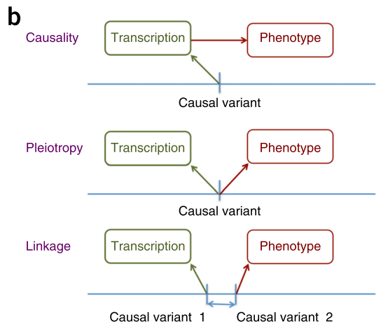
Three possible explanations of an association
It turns out that it is possible to filter out the “linkage” case. The paper suggested that if there is only one causal variant, the nearby region should have similar association signal. So, they proposed a hypothesis testing procedure to get rid of signal resulted from linkage. The following shows how they came up with the distribution under null hypothesis.
Let’s say there are $k$ loci in LD to the causal loci which is denoted as loci 0. For the causal loci and the $i$th locus, we have (consider $y \sim z$):
, where $h = 2p (1 - p)$ which is precisely $\var(z)$. So equation 7 follows. Intuitively, consider the following situation:
In this case, $b_{zy} = b_{xy} r_{zx} SE_x / SE_y$. Namely, if we know the dependency between $x$ and $z$, so does $x$ and $y$, then we can derive the dependency between $z$ and $y$. $r_{zx}$ indicates to what extent the effect size of $x$ on $y$ can be transferred to the one of $z$ on $y$. $SE_x / SE_y$ is a rescaling term. To match the same scale (namely $y$), $b \times SE$ should of the same scale for $z \sim y$ and $x \sim y$. Therefore, under the null hypothesis, $\hat{b}_{zy(i)}$ should have the same expected value. To make inference, we need some distribution of $\vec{b}_{zy}$, so we should know the variance/covariance as well.
- Side note:
I just found that the above derivation has a subtle drawback. It is that suppose we do
$\cov(\cdot, z_{(0)})$instead and do it carelessly, it will fail. The problem comes from the term$\cov(\epsilon_{(i)}, z_{(0)})$. From the derivation above, it seems to me that$z_{(0)}$and$z_{(i)}$are equivalent and interchangeable but it is really not the case. The graph above has pointed out such difference but in an implicit way. A more explicit illustration is the following:
The corresponding equations are:
, from which it is easy to see that
$\cov(\epsilon_{(i)}, z_{(0)}) \neq 0$
From the result of $\eqref{eq:1}$, we have:
, where \eqref{eq:2} follows from the fact that $r_{0i}$ and $\gamma_{0i}$ are simply the property of the locus 0 and locus i, so that $r_{0i} = \gamma_{0i}$. The same logic follows for $h$ and $\eta$.
This result implies that $\hat{d}_{i} := \hat{b}_{(i)} - \hat{b}_{(0)}$ has mean zero. Then, under the null, $(\hat{d}_{1}, ..., \hat{d}_k) \approx \mathcal{N}(0, R)$ (as stated in the text page 9 top left). $R$ is the variance/covariance matrix with entry $\cov(\hat{d}_i, \hat{d}_j)$.
From \eqref{eq:d} (as stated in equation 8), we need to compute $\cov(\hat{b}_{(i)}, \hat{b}_{(j)}), \forall i, j = 0, 1, ..., k$. The derivation of this term is sketched in the supplement part 3. The missing part seems unclear for me, so I derive it great details as follow.
The unclear thing is how to get $\E(g(\hat\theta))$ using Delta method. For $\var(g(\hat\theta))$, it is straight forward, but not so for the first order term because $\E(g(\hat\theta)) \approx g(\theta)$ is what we commonly use in practice. But if we take a closer look at Delta method, we will be sure that we can do more than this (see post about Delta method). That is to use higher order approximation.
\eqref{eq:3} is commonly used approximation and \eqref{eq:4} is a more “accurate” one. The corresponding multivariate version is simply:
, where $H(g(X))$ is the Hessian of $g$ evaluated at $\mu$ and $\Sigma_X$ is the variance/covariance matrix of $X$ and $\langle \cdot, \cdot \rangle$ is the matrix inner product. Now, we can apply this rule for deriving $\cov(\hat{b}_{(i)}, \hat{b}_{(j)})$.
\eqref{eq:6} is stated in supplement page 10. For an association signal, $\frac{\hat\beta}{\var(\hat\beta)}$ should be big (namely the $\chi^2$ statistic). Also, $\cov(\hat{b}_{zy(i)}, \hat{\beta}_{zy(i)}) = 0$. Therefore,
This result gives nothing more than the first order approximation. But it does matter for $\E(\hat{b}_{xy(i)}\hat{b}_{xy(j)})$. The intuition is that as more and more terms get involved, the first order approximation becomes worse and worse. So, in general, when too many terms involved, you need to be careful. If the (co)variance or Hessian is crazy, maybe it is a good idea to go beyond first order approximation.
It turns out that we need to compute $\cov(\hat{b}_{zy(i)}, \hat{b}_{zy(j)})$ and $\cov(\hat\beta_{zx(i)}, \hat\beta_{zx(j)})$. In the supplementary notes, it was stated as We know that the sampling correlation between the estimates of SNP effects equals to the LD correlation between the SNPs. But, again, this result is not intuitive to me. The following is a derivation of this:
Suppose $z$ has been standardized and the true effect size is $b$. Then $y = b z_0 + \epsilon$ where $z_0$ is the causal variant and $\epsilon$ is the error term. We have:
- Side note:
Note that \eqref{eq:sub2} seems conflict with \eqref{eq:varb}. But the difference is that \eqref{eq:varb} is for causal variant effect size estimator and \eqref{eq:sub2} is for the non-causal variants in LD. Intuitively, the association signal captured by non-causal variant comes from LD and only from LD. That’s why correlation of $\hat{b}$ matches exactly to correlation of $z$.
This proof stuck me from a long time. The confusing part is that I cannot formalize the underlying model in a proper way. At first, I tried:
I failed because it turns out that in this case the $A$ term will depend on the error term of $i$ and $j$. Essentially, this is not the correct underlying model of the problem. Neither $z_i$ nor $z_j$ have the real effect size well defined since they are not the causal variant. To make it physically make sense, it is necessary to consider $z_0$, the causal variant, somewhere in the calculation.
Also, a useful equation for deriving $\cov$ is:
This equation divides the problem into simpler and easier to deal with chunks, especially when $Y$ and $Z$ introduce dependency, which complicates the calculation. This equation can tease such dependency apart and work on them after simplifying the expression a bit.
After we obtain the distribution of $\hat{d}_1, ..., \hat{d}_k$, the normalized version is $z_i := \hat{d}_i / \sqrt{\var(\hat{d}_i)}$ with normalized (co)variance. The test statistic is constructed as $T_{HEIDI} = \sum_i z_i^2. The CDF of $T_{HEIDI}$ can be computed approximately (Satterthwaite or Saddlepoint as stated in the text).
Results in brief
In practice, they used blood eQTL data because of its large sample size. For each gene (only probe), they used the top associated cis-eQTL with HEIDI test to filter out linkage cases. For 5 complex traits, they identified 104 significant genes. Some insightful results are listed below:
- They pointed out that the loci which shows trait-associated gene signal (namely passed the tests in the paper) tends to be found in the future GWAS as the sample size increases. Second,
- SMR helps to pinpoint functionally relevant genes. In GWAS, many locus are close to multiple genes and SMR can distinguish them by considering whether the loci affects the gene expression.
- eQTL analysis are tissue-specific, but throughout the paper, they used blood eQTL results. They pointed out that many eQTL are shared across tissues, which benefits most by this strategy. But some tissue-specific eQTL is missed unavoidably. They showed that the signals identified in blood data were consistent with the results in brain data for schizophrenia GWAS (brain signal is weak due to power issue). But this indicates that SMR in unmatched tissue does not give fake signal. They did SMR with $x$ as expression in blood and $y$ as expression in brain for significant locus. They showed pleiotropic association as well. Also, the effect size learned from blood data can explain the same amount of variance in brain expression data as brain eQTL analysis did. These evidences showed that variants shared across tissues can be successfully captured by SMR even unrelated tissue eQTLs were used.
- Multiple tagging probes for a single gene is common in eQTL analysis. Probes tag the transcript and ideally we want every tag of the same gene gives consistent result, but it is not always the case (which might be significantly different from each other). They pointed out that such in-consistency may come from the fact that probes are tagging different types of transcripts from the same gene. But they failed to provide further evidence for this argument and they found that probes were not enriched in region close to transcription end site which is the place enriched for alternative splicing.
- HEIDI test assumes one causal variant per locus which may not be true in practice and non-pleiotropic variant may dilute the signal. So, they performed conditional analysis to overcome this issue. Not sure how they did this analysis. But I will read and post the note of the referred paper (see link). Added on 12/19/17: The idea of conditional analysis is to remove the effect of secondary variant in the region. Conditioning on the potential secondary variant, the effect size and HEIDI analysis were performed. This analysis can remove dilution effect caused by non-pleiotropic variant.
- Side note – the hypothesis test in 4)
Suppose
$\beta_{i1}, \beta_{j2}$are two effect size of $x \sim z$, where $i, j$ denote SNP index and $1, 2$ denote probe index. LS estimator is\hat\beta_{i1} = $z_i' x_1$and the same for $j2$ for standardized$z_i, z_j, x_1, x_2$. We have$\var(\hat\beta) = n \var(x) \var(z)$. And covariance is:
Discussion
HEIDI cannot distinguish linkage and pleiotropy if the two causal variants are in high LD (in this case, the data is not informative). To distinguish causality and pleiotropy, they proposed that multiple independent SNPs would help but it is a bit unclear how to construct the null distribution. Nonetheless, SMR provided a prioritized list of gene candidates for experimental validation. Furthermore, besides eQTL, other quantitative trait can be used, such as meQTL, pQTL, etc.